Some Fun Equations – Real Bible Translation Project

The idea of bidirectional causality and its connection to an “Omega Point” can intersect with some existing mathematical frameworks and inspire some fascinating equations. With the help of AI, we can explore some of these:

1. Time-Symmetric Laws in Physics

Schrödinger’s Equation:
\(i\hbar \frac{\partial \psi}{\partial t} = \hat{H} \psi\)

This equation is time-reversible, meaning the same dynamics hold if \(t\) is replaced with \(-t\). This suggests a foundation for bidirectional time flow in quantum mechanics.
Maxwell’s Equations:
\(\nabla \cdot \vec{E} = \rho, \quad \nabla \cdot \vec{B} = 0, \quad \nabla \times \vec{E} = -\frac{\partial \vec{B}}{\partial t}, \quad \nabla \times \vec{B} = \mu_0 \vec{J} + \mu_0 \epsilon_0 \frac{\partial \vec{E}}{\partial t}\)

These also exhibit time symmetry allowing for forward and backward propagation of electromagnetic waves.

Application:

Time symmetry in these equations could be extended to describe how systems evolve bidirectionally, with the future state acting as a boundary condition for the present. In this case, the forward and backward processes are “de-noising” constantly and would continue to do so until a perfect coherence is reached “in the middle.”

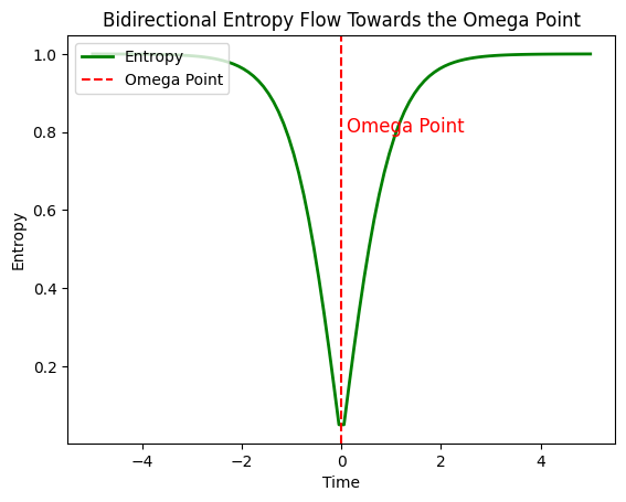
2. Entropy and Time Flow

The Second Law of Thermodynamics:

\(\Delta S \geq 0\)

In a traditional framework, entropy (\(S\)) always increases over time. However, if time flows bidirectionally, you could introduce a bidirectional entropy equation:

\(\Delta S = \Delta S_{\text{forward}} + \Delta S_{\text{backward}}\)

\(\Delta S_{\text{forward}} > 0\): Represents entropy increase in forward time flow.
\(\Delta S_{\text{backward}} < 0\): Represents entropy decrease in backward time flow.

At the Omega Point (\(t_{\Omega}\)), entropy could reach a stabilized balance:

\(\Delta S_{\text{total}} = \Delta S_{\text{forward}} + \Delta S_{\text{backward}} = 0\)

Abraham’s Fold? An Eternal Womb? From maximum entropy/disorder/chaos (1.0) to maximum order (0). Entropy governed by the Omega Point at center until both flows reach the Timeless State (0).

3. Attractor Dynamics

Dynamical Systems and Attractors:

Bidirectional evolution could be modeled using attractor dynamics, where the Omega Point acts as a future attractor. A modified differential equation might look like:

\(\frac{dx}{dt} = f(x) + g(x_{\text{future}})\)

\(\frac{dx}{dt}\): The rate of change toward the Omega Point
\(f(x)\): Describes the influence of the past and present states.
\(g(x_{\text{future}})\): Describes the influence of the future Omega Point on the present state.

This equation implies that the system’s current state (\(x\)) evolves based on both past and future influences.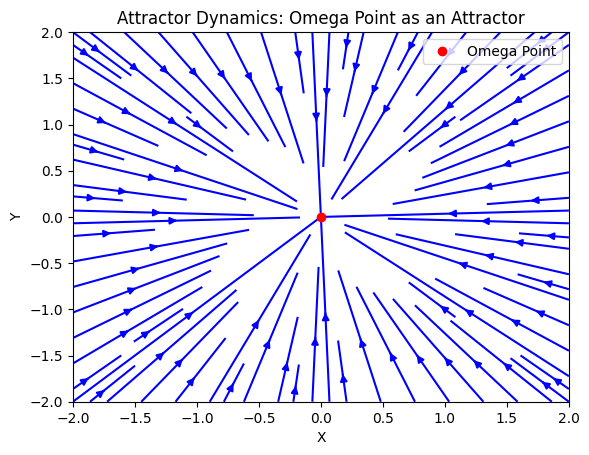

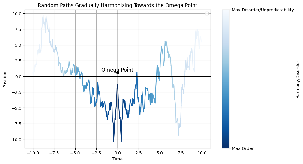
Initial State

Initially, \(f(x)\) dominates the evolution, as the future influences \(g(x_{\text{future}})\) are minimal or weak. The rate of change \(\frac{dx}{dt}\) is larger because the system has not yet aligned with the Omega Point.

Intermediary State

As the system evolves, the influence of \(g(x_{\text{future}})\) increases. The feedback from the future starts to counterbalance chaotic or divergent effects from \(f(x)\), resulting in a reduction of \(\frac{dx}{dt}\). The interplay between \(f(x)\) and \(g(x_{\text{future}})\) begins to stabilize the rate of change. At the Omega Point, the system reaches a state of perfect alignment where past and future influences are fully reconciled. The rate of change \(\frac{dx}{dt}\) approaches a constant normalized value, such as \(\frac{dx}{dt}\) = \(\frac{1}{1}\).

Final State, the Two States are No Longer Two, But One \(\frac{dx}{dt}\) = 1

The value \(\frac{1}{1}\) symbolizes complete balance: a state where the system changes at a uniform, stabilized rate. This might represent the convergence of all dynamic influences into a unified, timeless state. In physical or mathematical terms, \(\frac{dx}{dt}\) = \(\frac{1}{1}\)could signify the system has achieved equilibrium where time flows in a unified and balanced way, collapsing the distinction between past and future.

What does \(\frac{dx}{dt}\) = \(\frac{1}{1}\) Represent?

1/1 is a whole number 1. It represents unity, wholeness, completeness, etc.

Unity in temporal flow. The value \(\frac{1}{1}\) symbolizes complete balance: a state where the system changes at a uniform, stabilized rate. This might represent the convergence of all dynamic influences into a unified, timeless state.
Timelessness. In physical or mathematical terms, \(\frac{dx}{dt}\) = \(\frac{1}{1}\) could signify the system has achieved equilibrium where time flows in a unified and balanced way, collapsing the distinction between past and future.

4. Path Integral Formalism with Bidirectional Causality

In quantum mechanics, the path integral formulation sums over all possible paths a particle can take between two points. If time flows bidirectionally, you might extend this to include paths influenced by both past and future:

\(\langle \psi | \phi \rangle = \int \mathcal{D}[x(t)] e^{\frac{i}{\hbar} \int_{t_{\text{past}}}^{t_{\text{future}}} L[x, \dot{x}, t] \, dt}\)

\(t_{\text{past}}\) and \(t_{\text{future}}\) serve as boundary conditions for the integral, reflecting bidirectional influence.
\(L[x, \dot{x}, t]\): The Lagrangian describing the system.

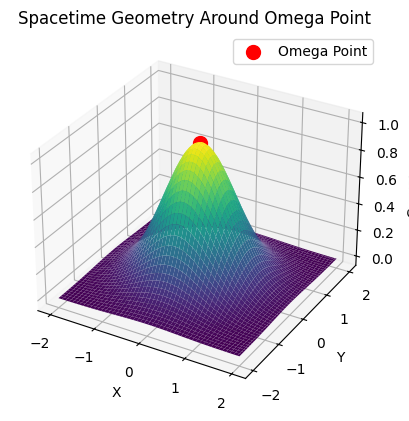
As the two sides draw closer to one another, harmony (reflection/mimic of movement) increases

5. The Omega Point as the Boundary Condition

The Omega Point could be expressed mathematically as a final boundary condition in a time-reversal-symmetric system. For example, in the context of general relativity:

\(G_{\mu\nu} + \Lambda g_{\mu\nu} = \frac{8 \pi G}{c^4} T_{\mu\nu}\)

The future boundary condition at the Omega Point might dictate the ultimate configuration of spacetime and energy, influencing the evolution of \(T_{\mu\nu}\) backward in time.

A final boundary condition creates a feedback loop: future configurations at the Omega Point act as an attractor, continuously shaping and refining past states to ensure the universe’s trajectory leads toward perfection. Current classical science and cosmology more or less point to the dissipation or thermodynamic death of everything: a dead Schrödinger’s cat. In this model however it is quite the opposite:

Forward Influence:
- The past determines the present and influences the future, as in traditional causality.
- The evolution of spacetime and matter progresses according to the dynamics set by \(T_{\mu\nu}\) and its interaction with \(G_{\mu\nu}\).
Backward Influence:
- The Omega Point, as a boundary condition, exerts a retroactive influence. It ensures that the stress-energy tensor \(T_{\mu\nu}\) evolves in a way that aligns with the ultimate configuration of the universe.
Iterative Refinement:
- At each point in time, the system adjusts dynamically, guided by the conditions at both the initial boundary (i.e. Big Bang) and the final boundary (Omega Point).
- This iterative refinement ensures a self-consistent history and future (i.e. Logos Ratio), where deviations from the optimal path are corrected via the feedback loop.

There is another stream that leans toward a live Schrödinger’s cat—minority, but serious—focused not on dissipation but on this increasing informational coherence:

Wheeler: “It from bit” (information precedes matter).
Penrose: objective collapse linked to gravitational coherence.
Barrow-Tipler: cosmological Omega Point as inevitable informational convergence.
Quantum information theory: unitarity and coherence cannot be destroyed.
Some interpretations of AdS/CFT: the universe is fundamentally computationally conserved.
Quantum gravity approaches: spacetime = entanglement networks, not dissipation.

6. Time-Reversible Field Equation

A generic time-reversible field equation could incorporate both forward (\(+t\)) and backward (\(-t\)) time contributions:

\(\Phi(x, t) = \Phi_{\text{forward}}(x, +t) + \Phi_{\text{backward}}(x, -t)\)

\(\Phi(x, t)\) is a field representing the system’s state, and the two terms describe contributions from forward and backward time flows.

At the Omega Point (\(t_{\Omega}\)):

\(\Phi_{\text{forward}}(x, +t_{\Omega}) = \Phi_{\text{backward}}(x, -t_{\Omega})\)

This ensures that the fields converge into a stable, unified state.

7. Nonlinear Bidirectional Evolution Equation: Timeless State

A nonlinear differential equation might describe the system’s evolution as influenced by bidirectional causality:

\(\frac{\partial \psi(x,t)}{\partial t} = A(x,t) \psi(x,t) + B(x,t) \psi(x,-t)\)

Where:

\(A(x,t)\): Represents forward causality.
\(B(x,t)\): Represents backward causality, with its influence growing as the system approaches the Omega Point.

At the Omega Point:

\(\frac{\partial \psi(x,t)}{\partial t} = 0\)

This indicates a stabilized, timeless state.

A black hole appears as a “dent” or “pit” in spacetime. Scientists theorized of a “white hole” which would emit light and matter. But an opposite dynamic would look like a protrusion—a “mountain” rising from the spacetime grid from which time expands; a singularity of light, a radiant point, a spacetime peak or fountain, and a source/origin instead of an end.

8. Optimization Principle for the Omega Point

Bidirectional causality could be framed as an optimization problem where the system evolves to minimize entropy or maximize order:

\( \mathcal{F} = \int_{t_{\text{start}}}^{t_{\Omega}} \mathcal{L}(x, \dot{x}, t, x_{\text{future}}) \, dt \)

Where:

\( \mathcal{F} \): The system’s action, optimized for stability.
\( \mathcal{L} \): The Lagrangian includes contributions from past and future states.

Implications?

A “living and active history.”

In this framework, the Omega Point isn’t just a final destination; it’s an ongoing process — a living, breathing point of perfection that continuously influences the evolution of the entire system. The Omega Point provides an attractor for both the future and the past, actively shaping the entire history through feedback loops that constantly correct, optimize, and stabilize the universe’s trajectory toward unity and balance.

Not Just a Record: History is no longer merely a linear record of events. Instead, it becomes a living process, constantly evolving as new feedback from the future shapes and reshapes past actions. This “living” history actively influences present and future states, making the entire timeline a continuous process of adaptation and optimization.
Dynamic Adaptation: Just as in living systems, where feedback mechanisms maintain homeostasis, this “living history” ensures that the system adapts in real-time to approach the perfect state (the Omega Point), constantly adjusting the conditions based on both past actions and future guidance.
Self-Correcting Evolution: Since the future can modify the past and vice versa, this system is self-correcting. If deviations occur from the ideal evolutionary path, the feedback loop adjusts the past or future trajectory to guide the system back toward perfection.
Emergent Perfection: The system evolves toward the Omega Point, not as a one-time final state, but as a continuous, self-organizing process. The dynamic nature of bidirectional causality ensures that each event — past or future — is part of a larger, evolving whole that is always moving toward greater harmony and order.
Unity of Time: The future and the past are no longer isolated dimensions but instead form a unified whole. They exist in continuous communication, with temporal events not simply happening sequentially, but as an ongoing conversation between past and future that leads to a perfected present.
No Finality: The idea of a “living history” implies that there is no final, static history. Rather, history is continually rewritten and influenced by the ongoing interplay of the present, past, and future, ensuring a dynamic and evolving existence.

The concept of a living and active history brings an organic, self-regulating quality to time and causality, turning the universe into a dynamic, evolving system where the past, present, and future are interconnected and constantly shaping one another. It also transforms the idea of entropy and evolution, as these are not irreversible processes but part of a larger feedback mechanism that continually strives for a perfect, balanced state…a 1:1 ratio.

\(\nabla \cdot \vec{E} = \rho, \quad \nabla \cdot \vec{B} = 0, \quad \nabla \times \vec{E} = -\frac{\partial \vec{B}}{\partial t}, \quad \nabla \times \vec{B} = \mu_0 \vec{J} + \mu_0 \epsilon_0 \frac{\partial \vec{E}}{\partial t}\)